Introduction

In medical epidemiology, prevalence is defined as the proportion of the population with a condition at a specific point in time (point prevalence) or during a period of time (period prevalence). [1] Prevalence increases when new disease cases are identified (incidence), and prevalence decreases when a patient is either cured or dies.  Many times, the period prevalence will provide a more accurate picture of the overall prevalence since period prevalence includes all individuals with the condition between two dates: old and new (incident) cases, as well as those who were cured or died during the period. [2][3]  

Clinically, prevalence is most commonly described as the percentage with the disease in the population at risk.   We commonly hear this in everyday discussion, and most find these references intuitive to interpret, such as "currently, X% of Americans were overweight or obese."  

Function

Prevalence = (Total number with disease) / (Population at risk for the disease)[2][4]

Alternatively, if the disease process tends to last a long time and both the incidence and cure/death rates are relatively stable then prevalence can be calculated based on the incidence and duration of disease.

• Prevalence = (Incidence) x (disease duration)

Let us use an example to examine and clarify prevalence.

Example 1

You talk to all 200 people in your town on a spring day and find 60 of them have allergy symptoms.  The point prevalence of allergies in your town would be 30% or 3 in 10 individuals calculated as:

• (60 people with allergy symptoms) / (200 people at risk) = 0.3 = 30%

You spend the next week interviewing all 1500 people in the next town over and find 300 people report allergy symptoms.  The period prevalence for the next town over is 20% for the week or 2 in 10 individuals calculated as:

• (300 people with allergy symptoms during the week) / (1500 people at risk) = 0.2 = 20%

Example 2

As stated previously, we can use the incidence and disease duration to calculate prevalence if both are relatively constant.

The annual incidence of the brain tumor glioblastoma is approximately 2.5 / 100,000 people annually in the United States.  The median survival at the time of diagnosis is approximately 15 months (1.25 years).  What is the prevalence of glioblastoma?

• Prevalence = (Incidence) x (disease duration)
• Incidence = 2.5 new cases / 100,000 people annually
• Disease duration = 1.25 years
• Prevalence = (2.5 cases / 100,000 people annually) x (1.25 years) = 3.125 cases / 100,000 people

Thus approximately 3.125 people out of every 100,000 individuals in the United States currently have a glioblastoma or approximately 10,125 people in the United States are currently living with the diagnosis of a glioblastoma.  This figure was calculated as:

• (3.125 cases / 100,000 people) x (324,000,000 people in the United States) = 10,125 cases of glioblastoma in the United States

It should be stressed that the second method is only valid if both the incidence and surival/disease duration are relatively constant.

Issues of Concern

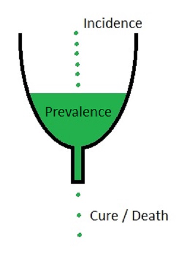
Prevalence is commonly confused with incidence.  Incidence is the rate of new cases or events during a specified time period for a population at risk whereas prevalence is the total cases present at one specific time, both new and old cases.  Incidence occurs when the new case is diagnosed, and each new case diagnosed increases the prevalence.  Prevalence decreases when the disease is cured, or the patient dies.  The cure for a disease or death of a patient does not affect the incidence of the disease whereas it decreases the prevalence.  In the image below incidence is the new additions to the reservoir, prevalence is the total in the reservoir, and cure/death decreases the reservoir.  Stated another way, the incidence is a measure of the risk of getting the disease during a specified time period whereas prevalence is a measure of how much burden of the disease there is in the population at one specific moment in time.[5][6]

A second common error with prevalence is not correctly defining the population at risk.  The total number of people living with ovarian cancer is estimated to be 0.13% of females (222,060 women living with ovarian cancer in the United States / 170,000,000 females in the United States).  If one were to make a mistake and use the total population of the United States instead of only females the prevalence would be incorrectly reported as 0.07%.  This 0.07% prevalence is not correct as only females are at risk, not all individuals.

Prevalence is also not static among different groups.  We will take two different examples, osteosarcoma and essential hypertension, and compare their prevalence stratified by age group.  Osteosarcoma tends to occur in the pediatric age group and has a second incidence peak in the elderly.  Osteosarcoma has approximately a 20% 10-year survival rate. Thus a pediatric patient diagnosed with osteosarcoma will likely no longer be alive in 10 years.  If there are few new cases in teenagers and adults, the prevalence will decrease as more individuals leave the disease group (by death or cure) than new cases are diagnosed.  Later in life, there is the second incidence peak where senior citizens start developing osteosarcoma at increasing rates.  This will add new cases to the osteosarcoma group, and thus the prevalence will increase in senior citizens corresponding to this second peak in incidence.

Essential hypertension, on the other hand, has an average life expectancy of decades after diagnosis.  As people get older, more individuals are newly diagnosed with essential hypertension (new incident cases), and thus the prevalence of essential hypertension increases with increasing age as we add the new diagnoses of essential hypertension to all of the old cases of essential hypertension still alive.

Clinical Significance

Prevalence is a measure of how common a disease process is found in a specified at-risk population at a specific time point or during a specified time period.  Prevalence is thus a measure of disease burden for the specified population, or how commonly someone with the disease will be encountered in the specified population.[2]

In biostatistics, prevalence could be considered similar to the pre-test probability.  That is, before any testing, the probability of a person in the specified population having the disease is the same as the prevalence of the disease in the population.  If the prevalence of a disease is 1% of the population, then we would expect approximately 1 in 100 people to have the disease before any testing.

Prevalence Impact on Positive Predictive Value (PPV) and Negative Predictive Value (NPV)

Prevalence thus impacts the positive predictive value (PPV) and negative predictive value (NPV) of tests.  As the prevalence increases, the PPV also increases but the NPV decreases.  Similarly, as the prevalence decreases the PPV decreases while the NPV increases.

For a mathematical explanation of this phenomenon, we can calculate the positive predictive value (PPV) as follows:

• PPV = (sensitivity x prevalence) / [ (sensitivity x prevalence) + ((1 – specificity) x (1 – prevalence)) ]

If we hold all values except for the prevalence the same then as prevalence increases the numerator will also increase for PPV.  In the denominator note the last term of “1 – prevalence.”  Thus as prevalence increases towards 100% (a value of one) the term “1 – prevalence” goes towards zero.  This drives the second part of the denominator, “(1 – specificity) x (1 – prevalence)”, to smaller and smaller values as prevalence increases.  Thus at a very high prevalence the value of “1 – prevalence” goes towards zero and the PPV equation reduces to:

• PPV = (sensitivity x prevalence) / [ (sensitivity x prevalence ) + ((1 – specificity) x (0)) ] =
• PPV = (sensitivity x prevalence) / [ (sensitivity x prevalence) + (0) ] =
• PPV = (sensitivity x prevalence) / (sensitivity x prevalence) = 1

Similarly we can write the negative predictive value (NPV) as follows:

• NPV = (specificity x (1 – prevalence)) / [ (specificity x (1 – prevalence)) + ((1 – sensitivity) x prevalence) ]

For the NPV as the prevalence increases (goes towards one) the term “1 – prevalence” becomes smaller making the numerator smaller.  In the denominator NPV has the same first term as the numerator, “specificity x (1 – prevalence)” which will also become smaller as the prevalence increases.  The second term in the denominator, “(1 – sensitivity) x prevalence” will increase as the prevalence increases.  As the prevalence comes very close to 100% we can write NPV as:

• NPV = (specificity x (1 – 1)) / [ (specificity x (1 – 1)) + ((1 – sensitivity) x 1) ] =
• (specificity x 0) / [ (specificity x 0) + (1 – sensitivity) ] =
• 0 / (0 + (1 – sensitivity)) = 0